Predictions & Data for this entry
| Model: std | climate: B, Cfa, Dfa, BSk | migrate: | phylum: |
| COMPLETE = 2.5 | ecozone: THn | food: biCi | class: |
| MRE = 0.062 | habitat: 0iTg, 0iTh, 0iTd | gender: Dg | order: |
| SMSE = 0.007 | embryo: Tt | reprod: O | family: |
Zero-variate data
| Data | Observed | Predicted | (RE) | Unit | Description | Reference |
|---|---|---|---|---|---|---|
| ab | 62 | 58.69 | (0.05344) | d | age at birth | guess |
| am | 2325 | 2318 | (0.002934) | d | life span | JoneBall1987 |
| Lb | 2.45 | 2.332 | (0.04819) | cm | SVL at birth | JoneBall1987 |
| Lp | 4.1 | 4.121 | (0.005226) | cm | SVL at puberty | JoneBall1987 |
| Li | 5.7 | 6.282 | (0.1021) | cm | ultimate SVL | JoneBall1987 |
| Wwb | 0.35 | 0.374 | (0.06863) | g | wet weight at birth | JoneBall1987 |
| Ri | 0.0274 | 0.02745 | (0.002069) | #/d | maximum reprod rate | JoneBall1987 |
Uni- and bivariate data
| Data | Figure | Independent variable | Dependent variable | (RE) | Reference |
|---|---|---|---|---|---|
| LW_f | 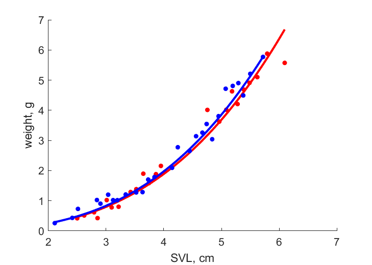 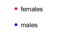 | SVL | weight | (0.08504) | Genn1974 |
| LW_m |   | SVL | weight | (0.0765) | Genn1974 |
| tL_fm | 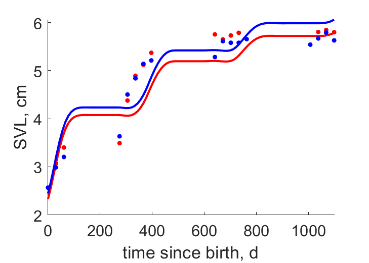  | time since birth | SVL | (0.07336) | JoneBall1987 |
Pseudo-data at Tref = 20°C
| Data | Generalised animal | Holbrookia maculata | Unit | Description |
|---|---|---|---|---|
| v | 0.02 | 0.01859 | cm/d | energy conductance |
| p_M | 18 | 521.4 | J/d.cm^3 | vol-spec som maint |
| k_J | 0.002 | 0.002 | 1/d | maturity maint rate coefficient |
| k | 0.3 | 0.03008 | - | maintenance ratio |
| kap | 0.8 | 0.9052 | - | allocation fraction to soma |
| kap_G | 0.8 | 0.8003 | - | growth efficiency |
| kap_R | 0.95 | 0.95 | - | reproduction efficiency |
Discussion
- T is assumed to vary as T(t) = 11+25*sin(2*pi*(t+100)/365) in C
- Males are assued to differ from females by {p_Am} only
Bibliography