Predictions & Data for this entry
| Model: abj | climate: MA | migrate: Ma | phylum: |
| COMPLETE = 2.5 | ecozone: MI, MPSW | food: bjPz, jiCi | class: |
| MRE = 0.045 | habitat: 0jMp, jiMm | gender: D | order: |
| SMSE = 0.004 | embryo: Mp | reprod: O | family: |
Zero-variate data
| Data | Observed | Predicted | (RE) | Unit | Description | Reference |
|---|---|---|---|---|---|---|
| ab | 5 | 5.048 | (0.009699) | d | age at birth | guess |
| am | 2920 | 2880 | (0.01371) | d | life span | guess |
| Lp | 8 | 8.057 | (0.007171) | cm | total length at puberty | guess |
| Li | 26 | 26.89 | (0.03413) | cm | ultimate total length | SabrAmin2015 |
| Wwb | 6.5e-05 | 6.677e-05 | (0.02724) | g | wet weight at birth | BrowSiva2003 |
| Wwi | 180 | 177.2 | (0.01554) | g | ultimate wet weight | fishbase |
| Ri | 328.8 | 331.5 | (0.008251) | #/d | max reproduction rate | guess |
Uni- and bivariate data
| Data | Figure | Independent variable | Dependent variable | (RE) | Reference |
|---|---|---|---|---|---|
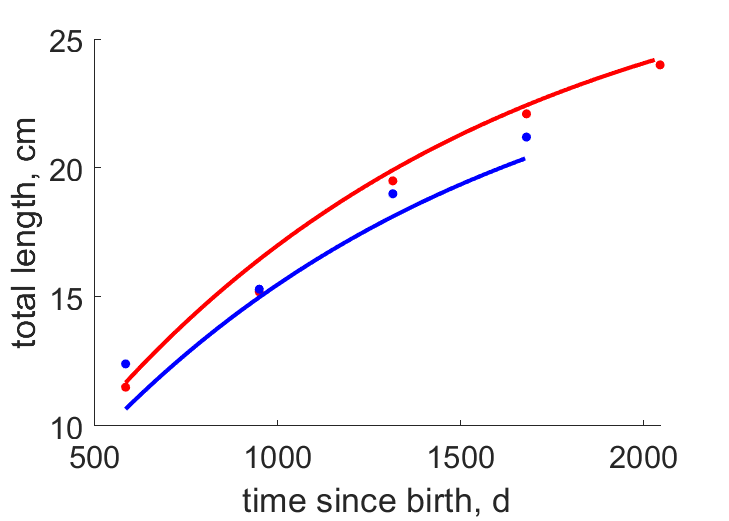
| tL_fm |   | time since birth | total length | (0.03926) | SabrAmin2015 |
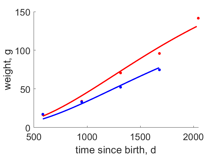
| tW_fm |   | time since birth | weight | (0.08045) | SabrAmin2015 |
Pseudo-data at Tref = 20°C
| Data | Generalised animal | Rogadius asper | Unit | Description |
|---|---|---|---|---|
| v | 0.02 | 0.0176 | cm/d | energy conductance |
| p_M | 18 | 8.347 | J/d.cm^3 | vol-spec som maint |
| k_J | 0.002 | 0.0004769 | 1/d | maturity maint rate coefficient |
| k | 0.3 | 0.3003 | - | maintenance ratio |
| kap | 0.8 | 0.95 | - | allocation fraction to soma |
| kap_G | 0.8 | 0.7962 | - | growth efficiency |
| kap_R | 0.95 | 0.95 | - | reproduction efficiency |
Discussion
- males are assumed to differ from females by {p_Am} only
- I had to add 1 yr to age estimates in tL and tW data to arrive at a good fit
Facts
- length-weight: Ww in g = 0.00525*(TL in cm)^3.04 (Ref: fishbase)
- known only from Coffs Harbor in northern New South Wales to Portland in Victoria, including Bass Strait and Tasmania (Ref: fishbase)
Bibliography